3 Numerical procedure

The evaluation of the free energy with temperature is not straightforward. Consequently, the anisotropy could be retrieved by calculating the average restoring torque in the equilibrium as a function of the constrained angles $\theta,\varphi$, which represents the polar and azimuthal angles of the magnetization from the easy axis. The torque acting on a system with mixed anisotropy (combination of uniaxial and cubic anisotropies) depends on the azimuthal and rotational angles in the following way:

$$\mathcal{T}(\theta,\varphi) = -K_{ua}^{eff}(T) \sin(2\theta) - \f... ...n^2(\theta)\biggl(\sin^4(\varphi)+\cos^4(\varphi)\biggr)-\cos^2(\theta)\Biggr).$$ (70)

If we evaluate the restoring torque at $\varphi =0$, we obtain that:

$$\mathcal{T}(\theta,0) = -K_{ua}^{eff}(T) \sin(2\theta) - \frac{1}{2}K_{ca}^{eff}(T)\sin(4\theta).$$ (71)

Thus, it is possible to obtain the values of anisotropy constants of the system and their behavior at different temperatures evaluating the torque curve.

In practice we first initialize the system with uniform magnetization in a direction of our choice $(\theta,\varphi)$, away from the anisotropy axes, where we expect a nonzero torque. Next we evolve the system by constrained Monte Carlo until the length of the magnetization reaches equilibrium. We then take a thermodynamic average of the torque over the number of constrained Monte Carlo ``sweeps''. We repeat at other orientations and we finally reconstruct the anisotropy constants from the angular dependence of the torque.

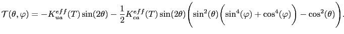
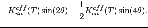
Torque curves for a generic system with uniaxial and cubic anisotropy are shown in Fig. 4.1. The symbols show the calculated torque and the curves are fitted to a $\sin\left(2\theta\right)$ dependence in the uniaxial case and to a $\sin(4\theta)$ dependence when the system has cubic anisotropy, where $\theta$ is the angle from the easy axis.

Figure 4.1: Simulated angular dependence of the restoring torque for a thin film with a simple cubic lattice, periodic boundary conditions and Tc close to $1100 K$, at temperatures 10 K, 100 K, and 500 K. (Left) Thin film with uniaxial anisotropy with easy axis parallel to Z axis. (Right) Thin film with cubic anisotropy with one of the easy axes parallel to Z axis.

The $\sin\left(2\theta\right)$ $\bigl[\sin(4\theta)\bigr]$ law is seen to hold at all temperatures for the case of uniaxial $\bigl[cubic\bigr]$ anisotropy and the fit of the restoring torque curves gives $K_{ua}^{eff}(T)$ $\bigl[K_{ca}^{eff}(T)\bigr]$.

In a situation like this, where all the torque curves have the same shape and the anisotropy is described by a single parameter, it is sufficient to compute the torque at 45 degrees in the uniaxial case and $\theta=22.5^\circ$ in the $xz$-plane for the cubic anisotropy case, where the maximum is known to occur. In more general cases it is necessary to compute the torque at several angular positions. Finally, with every new system it is prudent to verify the shape of the torque curves over many angles, both polar and azimuthal, before reducing the number of evaluated points.